I. Background
Currently, around 80 percent of American communities still adopt “single stream recycling” strategy to prevent more recyclable resources from landfills. While this strategy is applied to more and more American cities, the problem also appears. The proportion of contaminated recyclables increases from 7% to 25%, but also those “dirty” recyclable materials are less likely to get exported to other countries(i). The increasing difficulty to separate un-recyclable from recyclable requires that American cities experiment new strategies, such as dual stream recycling or multiple stream recycling strategies, to increase the recycling diversion rate, while the increasing amount of trash to be disposed daily in the city also challenge the efficiency of citywide recycling network.
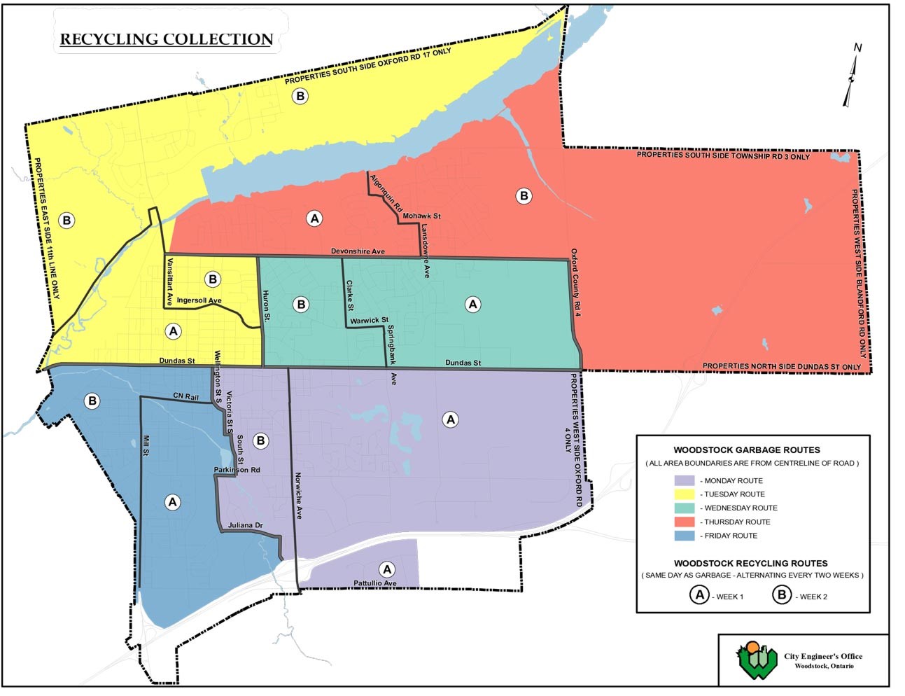
Besides, the efficiency of garbage collection is not well-considered. While your garbage may be collected or disposed by government, usually street department, or private disposal companies based on your housing type and your work place, most cities collect them by geographical area instead of area. Cities draw their own maps of garbage collection days based on population size so that every citizen know exactly when to drop their wrapped trash and recyclables through referencing the map and each collecting area has roughly similar population size. For example, city of Woodstock collects the garbage weekly and recycling bi-weekly. Besides, the city also has holiday garbage collection notice(ii, pic 1).
Fixed schedule can be convenient for citizens, but it loses efficiency. First, population density differs. Part of a collection area may have much higher population density than other parts, which requires more garbage truck routes or more garbage trips. Besides, predicting garbage number merely on the size of population usually overlooks the fact that different groups of people usually hold different attitude towards recycling. The number of recyclables collected from a large community that has low consciousness of recycling can be even lower than a small community with high enthusiasm in recycling. While collecting route can also be low efficient when stops of routes are assigned manually, lots of private companies have designed different method in improving the routing efficiency.
To summarize, most cities don’t have a “smart” mind in recycling. They don’t have a citywide model to test new recycling strategies on, and they also don’t know where effective strategies can be implemented in the city. All these problems in current solid waste recycling system have driven me to the topic of re-modeling, which focuses on introducing statistical methods in dealing with shortcomings in current recycling network.
II. Definition
a. Recycling Treatment Strategy
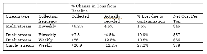
This term describes the overall strategies of recycling, including stream type and collection frequency. Stream type is measured by categories that the recyclables are divided into. There are three common steam types, including multi-stream, dual-stream and single-stream. Multi-stream means citizen are required to sort all kinds of recyclables according to government’s requirement. For example, Shinjuku in Japan has reclassified recyclable resources into 11 types, including newspaper&magazines, plastic containers, bottles, cans, spray cans, plastic PET bottles, disposable dry-cell batteries, cartons, white Styrofoam trays, collection of used small electronic devices and ink cartridges(iii.). Dual-stream means containers and paper/fiber need to be separated. Single-stream, mostly accepted by American cities, means that all recycling is sorted after collection. For frequency, cities usually collect garbage weekly and recyclables biweekly. A 2002 study has shown that both dual-stream recycling policy and multi-stream recycling policy are more economically beneficial and environmentally friendly (2002, EUREIKA RECYCLING, table 01). Adopting new recycling treatment strategies and apply them in the most suitable area becomes a core part of this project.
b. Socio-spatial Groups
This term is developed from social group. In social sciences, a social group is defined as two or more people who interact with one another, share similar characteristics and collectively have a sense of unity(iv.). The characteristics can include social interactions, common goals, interdependence in relation, different roles, group unity, etc(2010, Forsyth, Donelson,v.) . Socio-spatial groups, in my understanding, should be part of social groups, because most interactions, whether positive or negative, are spatially related. I would simplify the definition of socio-spatial group based on the topic of this project by saying “socio-spatial groups are groups that are spatially closed, socially similar, and share similar level of socio-economic characteristics”.
I believe using socio-spatial groups as the basis of my project is important, because socio-spatial groups incorporate spatial modeling problem with social-economic data. The abundant source in city economy, environment, demographics provide the possibility to build different models that may tackle the problem of city recycling strategies.
III. Data Source and Preprocessing
a. Socio-spatial Dataset
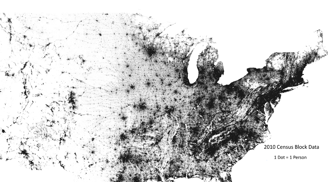
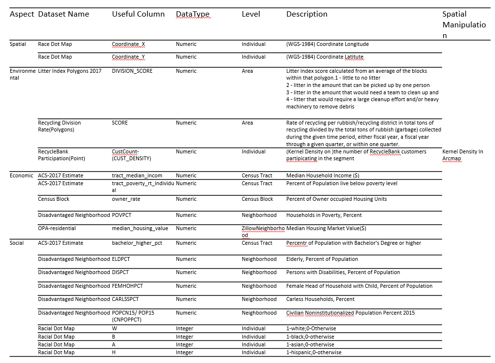
A very good data source to join other data on is the racial dot map from University of Virginia(pic 02). This dot map is based on block group race statistics and generate points randomly. Although this data set is a block based approximation of population distribution, it creates a modeling basis from individual perspective.
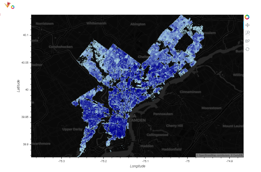
Use spatial join with Philadelphia city boundaries, we can generate a layer with population points that fall within the city boundary. This dataset contains around 1.5 million points(pic).
IV. Method
a. K-Means Clustering
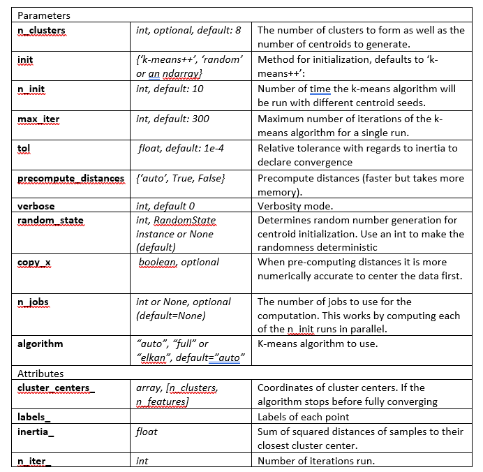
K-means clustering is an iterative algorithm that partitions the dataset into K pre-defined distinct non-overlapping subgroups where each data point belongs to only one group.(vi) Through each iteration, each point is assigned to its closest center, and newly formed groups generate new K centers for next iteration(pic 04).

This method is very useful in forming groups whose similarity is not limited to spatial approximation. Socio-economic factors can also be measurements in this algorithm. We will mainly use KMeans centence from scikit-learn package for this project. The parameters and attributes of scikit-learn KMeans algorithm includes(table 3):
b. PCA (Principal Component Analysis)
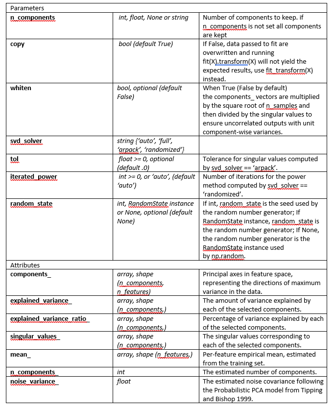
PCA will also be used if we want to reduce the linear dimensionality. For example, in part 3, we have introduced 20 variables for each data point. But when we are evaluating the influence of these 20 variables, we may want to combine some of the variables. Ideally, under the premise of not losing too much information of all 20 variables, we may want to reduce the dimensionality to 1. By reducing the dimensionality, we can introduce fewer variables without losing much of the original variance. This process sounds like the process of creating several aspects of land suitability from different source layers.
We will use PCA centences also from scikit-learn package for this project. The parameters and attributes of scikit-learn PCA algorithm includes(table 4):
c. Linear Regression Model and cross validation
We can also run different regression models on the dataset. The model that I select for this model is linear regression model. We also use linear model from scikit-learn.(x.)
V. Results
5.1 Import Necessary Packages and Dataset
This step imports all dataset that we will use for analysis. The data process include dropping all rows that has "-"s, beacause it mean no data is collected on the columns of these rows. There are also a lot of NaNs because not all datasets with shape have covered all area of the city. Therefore for points with NaNs, we decide to infill NaNs with column mean values.
The results can be used as important resource when we want to apply new treatment strategies.
import pandas as pd
import geopandas as gpd
import numpy as np
from sklearn.preprocessing import Imputer
# Read raw file from the folder
final_raw = pd.read_csv('Philly_recycling.csv')

# Get right columns
final_raw = final_raw[['easting', 'northing', 'W', 'B', 'A',
       'H', 'ELDPCT', 'POVPCT', 'DISPCT', 'FEMHOHPCT', 'CARLSSPCT', 'CNPOPPCT',
       'division_score', 'LANDVACPERCENTAGE', 'SCORE', 'market_value',
       'tract_median_incom', 'tract_poverty_rt_individual',
       'bachelor_higher_pct', 'owner_rate', 'CUST_DENSITY']]
# Delecting '-' from orginal dataset
final_raw = final_raw[final_raw['tract_median_incom'] != '-']
final_raw['tract_median_incom'] = final_raw['tract_median_incom'].astype(float)
final_raw = final_raw[final_raw['tract_poverty_rt_individual'] != '-']
final_raw['tract_poverty_rt_individual'] = final_raw['tract_poverty_rt_individual'].astype(float)
final_raw = final_raw[final_raw['bachelor_higher_pct'] != '-']
final_raw['bachelor_higher_pct'] = final_raw['bachelor_higher_pct'].astype(float)


# Imput column mean to NaN
imr = Imputer(missing_values = 'NaN', strategy = 'mean', axis = 0)
imr = imr.fit(final_raw)
imputed_data = imr.transform(final_raw.values)
final_raw = pd.DataFrame(imputed_data)
final_raw.columns = ['easting', 'northing', 'W', 'B', 'A',
       'H', 'ELDPCT', 'POVPCT', 'DISPCT', 'FEMHOHPCT', 'CARLSSPCT', 'CNPOPPCT',
       'division_score', 'LANDVACPERCENTAGE', 'SCORE', 'market_value',
       'tract_median_incom', 'tract_poverty_rt_individual',
       'bachelor_higher_pct', 'owner_rate', 'CUST_DENSITY']
5.2 KMeans and results
In this project, I simply select the cluster number of 30 because I set average cluster size could be around 50,000. Based on the total population number of 1.5 million in Philadelphia, it would be proper to set the number of clusters as 30.
# Import necessary libraries
import sklearn
from sklearn.cluster import KMeans
from sklearn.preprocessing import scale
# KMeans is sensitive to data scale, therefore we need to get all data into same scale
max = final_raw.max()
min = final_raw.min()
final_kmeans = final_raw - final_raw.min()
final_kmeans /= final_kmeans.max()
# Run the KMeans and fit it into the dataset
clustering = KMeans(n_clusters = 30, random_state = 0)
clustering.fit(final_kmeans)
# Getting labels for every point
final_kmeans_copy = final_kmeans.copy()
final_kmeans_copy['label']  = clustering.labels_
# Getting coordinates back
final_kmeans *= (max-min)
final_kmeans += min
# Add label array into orginal tabel to do spatial plot
final_kmeans['label'] = clustering.labels_
# Calculate number of points in each clusters using groupby().count()
count = final_kmeans_copy.groupby('label').count()
count = count.reset_index()
# Calculate average values of varaibles in each clusters using groupby().mean()
aver = final_kmeans_copy.groupby('label').mean()
aver = aver.reset_index()
import matplotlib
import matplotlib.pyplot as plt
%matplotlib inline
## Check different group size number
f = plt.bar('label','easting', data=count)

The resulting clusters are not equally divided, meaning that based on combinative consideration of spatial, environmental, economic and social factors, different clusters of socio-spatial groups have different sizes. The minimum group 14 has less than 20,000 persons, while the maximum group 13 is over 120,000.
# Check cluster performances on certain factors
fig, ax = plt.subplots(figsize=(28,13))
for i in range(1, 22):
    f = plt.subplot(3, 7, i)
    f.set_title(aver.columns[i])
    plt.bar(aver.columns[0], aver.columns[i],data=aver)

According to the averaged variable values, different groups also have different shape of distributions. For example, cluster 9 has a much higher density of recycle bank program participation than any other clusters. For bachelor's percent, around half of clusters has a higher level, and the other half of clusters have a lower level.
5.3 PCA and results
For PCA analysis, I mainly iterate through different numbers of principal analysis and see how much of the original varable is explained by different component choices. Normally the more principal components are chosen, the higher proportion of variance will be explained.
from sklearn.decomposition import PCA
from sklearn.preprocessing import StandardScaler

## standard-scaling the data
final = np.matrix(final_raw)
band = []
for i in range(final.shape[1]):
    scaler = StandardScaler()
    c = scaler.fit_transform(final[:,i].reshape(-1,1))
    band.append(c)
final = np.stack(band, axis = -1).reshape((1517884,21))


X_forExploringPCA = final.copy()
pca_model = PCA(n_components = 20)
pca_model.fit(X_forExploringPCA)
variance = pca_model.explained_variance_ratio_ #calculate variance ratios

var = np.cumsum(np.round(pca_model.explained_variance_ratio_, decimals=3)*100)
var #cumulative sum of variance explained with [n] features

plt.ylabel('% Variance Explained')
plt.xlabel('# of Features')
plt.title('PCA Analysis')
plt.axhline(y= 90)
plt.style.context('seaborn-whitegrid')
plt.plot(var)

We can see that when the number of features is higher tha 11, more than 90% of original variance can be explained. We usually don't know how to interprete the meaning of these new components in real life, because they are mixed combination of our original variables, but they can be useful in modeling, especially when the number of observations is small.
VI. Application
6.1 Finding spatial distribution of target groups for new treatment strategy implementation and designing the route
As is mentioned in the previous parts, the result of KMeans clustering has shown that cluster 9 has a very high density of recyclie bank participation than any other groups. This mean this socio-spatial groups may be more interested in participating programs of recycling with rewards. We can test new treatment strategies, such as testing multi-stream recycling strategy on this group to see if it do work. We can look at where this group distributes on space.
# We can also plot out the clusters to see hwo points in different clusters are distributed
# First, convert dataframe into geodataframe
from shapely.geometry import Point
final_kmeans['geometry'] = final_kmeans.apply(lambda row: Point(row['easting'],row['northing']), axis = 1)
# Save the point file as geojson
crs = {'init':'epsg:3857'} #http://www.spatialreference.org/ref/epsg/2263/
final_kmeans = gpd.GeoDataFrame(final_kmeans, crs=crs, geometry=final_kmeans['geometry'])
# Get basic Philadelphia Zip Codes
# base URL
url = "https://services.arcgis.com/fLeGjb7u4uXqeF9q/arcgis/rest/services/Zipcodes_Poly/FeatureServer/0/query?outFields=*&where=1%3D1"
# specif y GeoJSON format
url += "&f=geoJSON"
zip_codes = gpd.read_file(url)
zip_codes = zip_codes.to_crs(epsg=3857)
# Now Plot label 9 points on Philadelphia zip codes
ax = zip_codes.to_crs(epsg=3857).plot(facecolor='black', edgecolor='white', figsize=(20, 20))
ax.set_facecolor('black')
final_kmeans[final_kmeans['label'] == 9].to_crs(epsg=3857).plot(ax=ax, markersize=20, alpha = 0.3, color='orange')

The map above shows that the target group mainly distributes on West Philadelphia and Southwest Philadelphia. Since it is not a holistic group in space, the city can test new stream type by asking group member to get ready for it and opening a test routes for it. We can keep on using pure spatial KMeans to assign collecting stops for these people.
# Getting group 9
final_group9 = final_kmeans[final_kmeans['label'] == 9][['easting','northing']]
# Run the KMeans and fit it into the dataset, suppose each collecting stops will take care of 500 recyclers, we are running
# a new KMeans clustering of n_clusters = 80
clustering = KMeans(n_clusters = 80, random_state = 0)
clustering.fit(final_group9)
# Getting labels for every point
final_group9['label']  = clustering.labels_
# Getting centers
center = pd.DataFrame(clustering.cluster_centers_)
center.columns = ['easting','northing']
center['geometry'] = center.apply(lambda row: Point(row['easting'],row['northing']), axis = 1)
center = gpd.GeoDataFrame(center, crs=crs, geometry=center['geometry'])
ax = zip_codes.to_crs(epsg=3857).plot(facecolor='black', edgecolor='white', figsize=(20, 20))
ax.set_facecolor('black')
center.to_crs(epsg=3857).plot(ax=ax, markersize=20, alpha = 0.7, color='orange')
center['x'] = center.to_crs(epsg=4326).geometry.x
center['y'] = center.to_crs(epsg=4326).geometry.y
center.to_csv('center.csv')

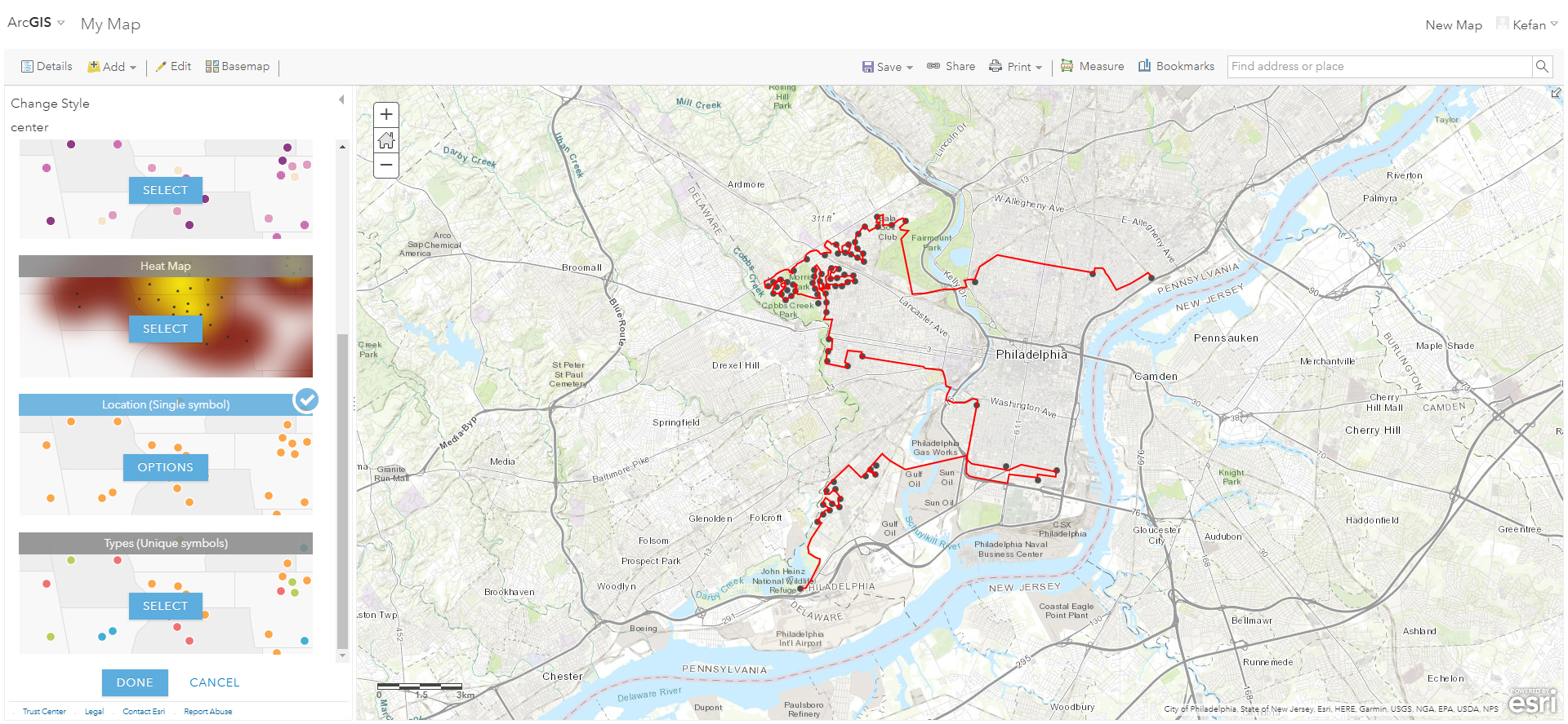
After generating the stops, we can easily expoted into a shapefile and generate shortest path using ArcGIS Online's network analysis function (pic 5).
6.2 Evaluating the urgency of requiring enhanced treatment strategy
We can also build models to evaluate the need of new treatment strategy based on score of litter index survey. As is shown in the variable description, this index measure the number of litter that influence the street view. The higher the score, the more litter on streets. This index measures the urgency level of getting new treatment strategy to control the influence from litter. We can sort average scores of this index and look at where high score groups and low score groups distributes. Based on our settings of colors, blue and aqua groups will have a cleaner area in their surroundings, while orange and red groups are in urgent need to clean surrounding trash.
# Sort Groups that has the lowest division scores (The groups perform well in maintaining their surrounding environment)
list_top = aver.sort_values(by = ['division_score'])['label'].tolist()
# Now Plot targeted group points on Philadelphia zip codes
ax = zip_codes.to_crs(epsg=3857).plot(facecolor='black', edgecolor='white', figsize=(20, 20))
color_list = ['blue'] * 5 + ['aqua'] * 5 + ['ivory'] * 5 + ['lime'] * 5 + ['orange'] * 5 + ['red'] * 10
ax.set_facecolor('black')
for num in range(30):
    final_kmeans[final_kmeans['label'] == list_top[num]].to_crs(epsg=3857).plot(ax=ax, markersize=20, alpha = 0.3, color = color_list[num])

Based on the distribution of different colored groups, it is obvious that central north Philadelphia and west Philadelphia performs badly in maintaining their surrounding street environment. This could suggest municipality increase the frequency of street cleaning, or increase the punishment of public littering. Compared to orange and red area, northeastern Philadelphia and northwestern Philadelphia has a better street environment.
6.3 Buidling prediction model on recycle bank enthusiamsm
We can also use this dataset to test to build a prediction model. Even though we don't have a dependent variable that directly measures current recycling efficiency, we still can explore the possibility of using model to predict the performance of certain variables. For example, we can build a linear regression mdoel to predict people's willing to participate in recycle bank.
from sklearn import datasets, linear_model
from sklearn.model_selection import train_test_split

# we will use ['W', 'B', 'A', 'H', 'ELDPCT', 'POVPCT', 'DISPCT', 'FEMHOHPCT', 'CARLSSPCT', 'CNPOPPCT','division_score', 'LANDVACPERCENTAGE', 'SCORE', 'market_value','tract_median_incom', 'tract_poverty_rt_individual', 'bachelor_higher_pct', 'owner_rate']

x = np.concatenate((np.matrix(final_raw)[:,0:2], final[:,2:19]), axis = 1)

y = final[:,20]

X_train, X_test, y_train, y_test = train_test_split(x, y, test_size=0.3)
model = lm.fit(X_train[:,2:], y_train)
predictions = lm.predict(X_test[:,2:])
print("Explained variance in test set: ", model.score(X_test[:,2:], y_test),"; Explained variance in training set: ", model.score(X_train[:,2:], y_train))
As we can see, the model that the prediction on training set has a very low score, which means only a small proportion of the variance of dependent variable is explained by the model. However, considering the huge number of observations, the performance of this model is not bad. Besides, the model performance in training set and test set is close, which means this model is less likely to be overfitting.
We can further explore the error of this model by plotting them out on the map.
error = np.concatenate((X_test[:,:2], (predictions - y_test).reshape(-1,1)), axis = 1)
error = pd.DataFrame(error)
error.columns = ['easting','northing','residual']
error['geometry'] = error.apply(lambda row: Point(row['easting'],row['northing']), axis = 1)
error = gpd.GeoDataFrame(error, crs=crs, geometry=error['geometry'])
ax = zip_codes.to_crs(epsg=3857).plot(facecolor='black', edgecolor='white', figsize=(20, 20))
ax.set_facecolor('black')
def get_color(x):
    if x > 0:
        return 'blue'
    else:
        return 'red'
error['color'] = error['residual'].apply(lambda x: get_color(x))

# Plot overestimate points
error[error['residual'] >= 0].to_crs(epsg=3857).plot(ax=ax, markersize=20, alpha = 0.7, color='orange')

ax = zip_codes.to_crs(epsg=3857).plot(facecolor='black', edgecolor='white', figsize=(20, 20))
ax.set_facecolor('black')
# Plot underestimate points
error[error['residual'] <0].to_crs(epsg=3857).plot(ax=ax, markersize=20, alpha = 0.7, color='aqua')

Comparing the two plots, most areas in the city have both underestimate points and overestimate points. The more interesting areas that are worth investigating are Overbook, Olney, Chestnut Hill and Roxborough. The model tend to underestimate the enthusiasm of groups in participating in recycle bank program, therefore these areas have potentials in promoting more recycle bank activities or they may be more proactive than the model would expect.
VII. Conclusion and discussion
This projects mainly explores how the city could deal with current recycling network problems from the perspective of data. The introduction of socio-spatial group dataset provide a way of incorporating spatial problems with more detailed data from multiple aspects, including envirmental, economic and social factors. The large number of data rows creates huge potential for more variables to be intrudced with little worry of overfitting. Compared to traditional method of spatial evaluation, the process of KMeans classification is value-neutral, which means we can have our preference of cluster choice after classification.
However, these methods also have their own limitation. First, different datasets have different projection system and geographical base. Not all citywide dataset is as specific as recording information on invidual level. Even the race dot map is calculated on block level. The lack of data on recycling measurements also makes it hard to build models on. Last but not least, the interpretation of certain methods can be difficult.
Appendix:
a. Reference
i.The era of easy recycling may be coming to an end. https://fivethirtyeight.com/features/the-era-of-easy-recycling-may-be-coming-to-an-end/
ii.City Of Woodstock. https://www.cityofwoodstock.ca/en/residential-services/collection-schedule-and-map.aspx
iii.Shinjuku City Official Website. http://www.foreign.city.shinjuku.lg.jp/en/seikatsu/seikatsu_2/
iv.Turner, J.C. (1982). Tajfel, H. (ed.). "Towards a cognitive redefinition of the social group". Social identity and intergroup relations. Cambridge: Cambridge University Press: 15–40.
v.Forsyth, Donelson, R. (2010). Group Dynamics, Fifth Edition. Belmont, CA: Wadsworth, Cengage Learning.
vi.Imad Dabbura, https://towardsdatascience.com/k-means-clustering-algorithm-applications-evaluation-methods-and-drawbacks-aa03e644b48a
vii.KMeans Clustering https://en.wikipedia.org/wiki/K-means_clustering#/media/File:K-means_convergence.gif
viii.Sklearn.cluster.KMeans https://scikit-learn.org/stable/modules/generated/sklearn.cluster.KMeans.html
ix.Sklearn.cluster.PCA https://scikit-learn.org/stable/modules/generated/sklearn.decomposition.PCA.html
x. Sklearn.linear_model.LinearRegression. https://scikit-learn.org/stable/modules/generated/sklearn.linear_model.LinearRegression.html
b. Data Collection Code
Please re-run the code from another jupyter notebook (The following code is only for displaying)
### Advanced Topics in GIS - Kefan Long#
## Appendix - Tabular Data Collection

# Pre-installed or Import Packages
import pandas as pd
import geopandas as gpd
import numpy as np
import cartopy.crs as ccrs
import datetime
import geocoder
import matplotlib.pyplot as plt
import dask.array as da
import dask.dataframe as dd
from shapely.geometry import Polygon, Point, MultiPoint

import scipy

# Pre-installed or Import Packages2
!pip install simpledbf

### Part 1. Collecting Data ###

1.1 Philadelphia Population Points Data
1.1.1 Manipulating Data From US Race Dot Map

df = dd.read_parquet('C:/Users/Kevin Long/Desktop/19Spring/CPLN-691/week-7-master/data/census2010.parq')
df = df.persist()

df.head()

# Importing the coordinate of different cities
from datashader.utils import lnglat_to_meters as webm

USA           = ((-124.72,  -66.95), (23.55, 50.06))
LakeMichigan  = (( -91.68,  -83.97), (40.75, 44.08))
Chicago       = (( -88.29,  -87.30), (41.57, 42.00))
Chinatown     = (( -87.67,  -87.63), (41.84, 41.86))
NewYorkCity   = (( -74.39,  -73.44), (40.51, 40.91))
LosAngeles    = ((-118.53, -117.81), (33.63, 33.96))
Houston       = (( -96.05,  -94.68), (29.45, 30.11))
Austin        = (( -97.91,  -97.52), (30.17, 30.37))
NewOrleans    = (( -90.37,  -89.89), (29.82, 30.05))
Atlanta       = (( -84.88,  -84.04), (33.45, 33.84))
Philly        = (( -75.28,  -74.96), (39.86, 40.14))


x_range,y_range = [list(r) for r in webm(*Philly)]
plot_width  = int(900)
plot_height = int(plot_width*7.0/12)

# Get Philadelphia Points
df_philly = df[((df['easting']> x_range[0]) & (df['easting'] < x_range[1]) & (df['northing'] > y_range[0]) & (df['northing'] < y_range[1]))]

# Persist and get stored
df_philly_pd = df_philly.compute()

philly_dot = df_philly_pd.reset_index()[['easting','northing','race']]

philly_dot.describe()

philly_dot.to_csv("philly_dot.csv")

philly_dot = pd.read_csv("philly_dot.csv")

from shapely.geometry import Point
# Convert Array to Multipoint
philly_dot['geometry'] = philly_dot.apply(lambda row: Point(row['easting'],row['northing']),axis = 1)

# Save the point file as geojson
crs = {'init':'epsg:3857'} #http://www.spatialreference.org/ref/epsg/2263/
philly_dot_gs = gpd.GeoDataFrame(philly_dot, crs=crs, geometry=philly_dot['geometry'])

1.1.2 Philadelphia City Bound

url = "http://data.phl.opendata.arcgis.com/datasets/405ec3da942d4e20869d4e1449a2be48_0.geojson"
city_bound = gpd.read_file(url)
city_bound = city_bound.to_crs(epsg=3857)
city_bound.plot()

philly_dot_gs.describe()

zip = gpd.sjoin(philly_dot_gs, city_bound, op = 'within')

len(zip)

type(zip)

zip.columns

zip = zip[['Unnamed: 0','easting','northing','race','geometry']]

zip.columns = ['index','easting','northing','race','geometry']

zip.head()

zip['W'] = zip.apply(lambda row: 1 if row['race'] == 'w' else 0 ,axis = 1)

zip['B'] = zip.apply(lambda row: 1 if row['race'] == 'b' else 0 ,axis = 1)
zip['A'] = zip.apply(lambda row: 1 if row['race'] == 'a' else 0 ,axis = 1)
zip['H'] = zip.apply(lambda row: 1 if row['race'] == 'h' else 0 ,axis = 1)

color_key = {'w':'aqua', 'b':'lime',  'a':'red', 'h':'fuchsia', 'o':'yellow' }

def create_image(longitude_range, latitude_range, w=plot_width, h=plot_height):
    x_range, y_range = webm(longitude_range, latitude_range)

    # setup the canvas
    cvs = ds.Canvas(plot_width=w, plot_height=h, x_range=x_range, y_range=y_range)

    # aggregate, but this time count the "race" category
    agg = cvs.points(df, 'easting', 'northing', ds.count_cat('race'))

    # shade, using our color key
    img = tf.shade(agg, color_key=color_key, how='eq_hist')

    return tf.set_background(img, 'black')


import holoviews as hv
import geoviews as gv
from holoviews.operation.datashader import datashade
hv.extension("bokeh")

points = hv.Points(zip[['easting','northing']], kdims=['easting', 'northing'])

# shaded
census = datashade(points).opts(width=900, height=600)

# background tile
bg = gv.tile_sources.CartoDark

bg * census

# Write to local directory
zip.to_csv("dot.csv")

1.2 Get Street

# Get Street Centerline
# url3 = 'http://data.phl.opendata.arcgis.com/datasets/ab9e89e1273f445bb265846c90b38a96_0.geojson'
# street = gpd.read_file(url3)
# street = building.to_crs(epsg = 3857)

street_center = gpd.read_file('./env/Street_Centerline.geojson')
street_center = street_center.to_crs(epsg = 3857)

len(street_center)

1.3 Census Block for enconomic Data

# Get census tract
# url4 = 'http://data.phl.opendata.arcgis.com/datasets/8bc0786524a4486bb3cf0f9862ad0fbf_0.geojson'
# tract = gpd.read_file(url4)
# tract = tract.to_crs(epsg=3857)

tract = gpd.read_file('Census_Tracts_2010.geojson')
tract = tract.to_crs(epsg = 3857)
tract.plot()

# Get census block group
# url5 = 'http://data.phl.opendata.arcgis.com/datasets/8bc0786524a4486bb3cf0f9862ad0fbf_0.geojson'
# block = gpd.read_file(url5)
# block = tract.to_crs(epsg=3857)

block = gpd.read_file('Census_Block_Groups_2010.geojson')
block = block.to_crs(epsg = 3857)
block.plot()

1.4 Get other useful dataset with shapefile

# Get litter index for street
# url6 = 'https://phl.carto.com/api/v2/sql?q=SELECT+*+FROM+litter_index_lines&filename=litter_index_lines&format=geojson&skipfields=cartodb_id'
# litter = gpd.read_file(url6)
# litter = litter.to_crs(epsg=3857)

litter = gpd.read_file('./env/Street_Centerline.geojson')
litter = litter.to_crs(epsg=3857)
litter.plot()

litter.head()

litter.columns

# Keep Useful Information
litter = litter[['CLASS','STNAME','geometry']]
litter.head()

# Get litter index for polygon
# url7 = 'https://phl.carto.com/api/v2/sql?q=SELECT+*+FROM+litter_index_polygon&filename=litter_index_polygon&format=geojson&skipfields=cartodb_id'
# litter = gpd.read_file(url6)
# litter = litter.to_crs(epsg=3857)

litter_area = gpd.read_file('./env/litter_index_polygon.geojson')
litter_area = litter_area.to_crs(epsg=3857)
litter_area.plot()

litter_area.head()

# Keep useful information
litter_area = litter_area[['division_num','division_score','geometry']]
litter_area.head()

# Get litter index survey
# url8 = 'https://phl.carto.com/api/v2/sql?q=SELECT+*+FROM+litter_index_survey&filename=litter_index_survey&format=geojson&skipfields=cartodb_id'
# litter_survey = gpd.read_file(url8)
# litter_survey = litter_survey.to_crs(epsg=3857)

litter_2017survey = gpd.read_file('./env/litter_index_survey.geojson')
litter_2017survey = litter_2017survey[litter_2017survey.geometry.notnull()]
litter_2017survey = gpd.GeoDataFrame(litter_2017survey, crs = {'init':'epsg:4326'},geometry = 'geometry')

litter_2017survey = litter_2017survey.to_crs(epsg = 3857)

# Keep only the useful information
litter_2017survey = litter_2017survey[['litter_count','rating','geometry']]
litter_2017survey.head()

# Get recycling diversion rate polygons
# url9 = 'http://data.phl.opendata.arcgis.com/datasets/79c1c68097e641208ca7041251a87067_0.geojson'
# recycle_diver_rate = gpd.read_file(url9)
# recycle_diver_rate.to_crs(epsg = 3857)

# Get recycling diversion rate polygons
recycle_diver_rate = gpd.read_file('./env/Recycling_Diversion_Rate.geojson')
recycle_diver_rate = recycle_diver_rate.to_crs(epsg = 3857)
recycle_diver_rate.head()

# Get wire basket location
# url10 = 'http://data.phl.opendata.arcgis.com/datasets/5cf8e32c2b66433fabba15639f256006_0.geojson'
# wire_basket = gpd.read_file(url10)
# wire_basket = wire_basket.to_crs(epsg = 3857)

wire_basket = gpd.read_file('./env/WasteBaskets_Wire.geojson')
wire_basket = wire_basket.to_crs(epsg = 3857)
wire_basket.head()

# Get recycle bank participation
# url11 = 'https://phl.carto.com/api/v2/sql?q=SELECT+*+FROM+recyclebank_participation&filename=recyclebank_participation&format=geojson&skipfields=cartodb_id'
# recycle_bank = gpd.read_file(url11)
# recycle_bank = recycle_bank.to_crs(epsg = 3857)

recycle_bank = gpd.read_file('./env/recyclebank_participation.geojson')
recycle_bank = recycle_bank.to_crs(epsg = 3857)
recycle_bank.head()

# Get building demolition
# url12 = 'https://phl.carto.com/api/v2/sql?q=SELECT+*+FROM+li_demolitions&filename=li_demolitions&format=geojson&skipfields=cartodb_id'
# building_demo = gpd.read_file(url12)
# building_demo = building_demo.to_crs(epsg = 3857)

building_demo = gpd.read_file('./env/li_demolitions.geojson')
building_demo = building_demo[building_demo.geometry.notnull()].to_crs(epsg = 3857)
building_demo.head()

# Get Shooting Victims
# url13 = 'https://phl.carto.com/api/v2/sql?q=SELECT+*+FROM+shootings&filename=shootings&format=geojson&skipfields=cartodb_id'
# shooting = gpd.read_file(url13)
# shooting = shooting.to_crs(epsg = 3857)

shooting = gpd.read_file('./socio/shootings.geojson')
shooting = shooting[shooting.geometry.notnull()].to_crs(epsg = 3857)
shooting.head()

# Get registred community organization
# url14 = 'http://data.phl.opendata.arcgis.com/datasets/efbff0359c3e43f190e8c35ce9fa71d6_0.geojson'
# organization = gpd.read_file('url14')
# organization = organization.to_crs(epsg = 3857)

# Get registred community organization
organization = gpd.read_file('./socio/Zoning_RCO.geojson')
organization = organization.to_crs(epsg = 3857)
organization.plot()

organization.head()

# Get bike network
# url15 = 'http://data.phl.opendata.arcgis.com/datasets/b5f660b9f0f44ced915995b6d49f6385_0.geojson'
# bike_network = gpd.read_file(url15)
# bike_network = bike_network.to_crs(epsg = 3857)

# Get bike network
bike_network = gpd.read_file('./socio/Bike_Network.geojson')
bike_network = bike_network.to_crs(epsg = 3857)
bike_network.plot()

# Get Potential Disadvantage indicator of neighborhood
# url16 = 'http://dvrpc-dvrpcgis.opendata.arcgis.com/datasets/882f8929b121417fb53009f865335c48_0.geojson'
# dis_indicator = gpd.read_file(url16)
# dis_indicator = dis_indicator.to_crs(epsg = 3857)

# Get Potential Disadvantage indicator of neighborhood
dis_indicator = gpd.read_file('./socio/DVRPC_2015_Indicators_of_Potential_Disadvantage.geojson')
dis_indicator = dis_indicator.to_crs(epsg = 3857)
dis_indicator.plot()

from shapely.geometry import Point

dis_indicator.columns

dis_indicator.head()

# Get data from 2017 real eatate
from pyrestcli.auth import NoAuthClient
from carto.sql import SQLClient

API_endpoint = "https://phl.carto.com"
sql_client = SQLClient(NoAuthClient(API_endpoint))
table_name = "RTT_SUMMARY"
query = "SELECT * FROM %s WHERE display_date >= '2017-01-01'" %table_name
transfer_from_2017 = sql_client.send(query, format='geojson')

transfer_from_2017 = gpd.GeoDataFrame.from_features(transfer_from_2017, crs = {'init':'epsg:4326'})

transfer_from_2017.columns

transfer_from_2017=transfer_from_2017[['geometry']]

transfer_from_2017.to_csv('./eco/transfer_from_2017.csv')

# Get Vacancy Property Ratio Indicator( Building and Land)
# url17 = 'http://data-phl.opendata.arcgis.com/datasets/35ee75560f3743b0bf832da2d977af43_0.geojson'
# building_vacan_rate = gpd.read_file(url17)
# building_vacan_rate = building_vacan_rate.to_crs(epsg=3857)

# Get Vacancy Property Ratio Indicator( Building and Land)
building_vacan_rate = gpd.read_file('./eco/Vacant_Block_Percent_Building.geojson')
building_vacan_rate = building_vacan_rate.to_crs(epsg=3857)

building_vacan_rate.head()

# Get Vacancy Property Ratio Indicator( Building and Land)
# url18 = 'http://data-phl.opendata.arcgis.com/datasets/35ee75560f3743b0bf832da2d977af43_0.geojson'
# land_vacan_rate = gpd.read_file(url18)
# land_vacan_rate = land.to_crs(epsg=3857)

# Get Vacancy Property Ratio Indicator( Building and Land)
land_vacan_rate = gpd.read_file('./eco/Vacant_Block_Percent_Land.geojson')
land_vacan_rate = land_vacan_rate.to_crs(epsg=3857)

land_vacan_rate.head()

url = "https://raw.githubusercontent.com/MUSA-620-Spring-2019/week-3/master/data/opa_residential.csv"
data = pd.read_csv(url)
data.head()

data['Coordinates'] = data.apply(lambda row : Point(row['lng'], row['lat']), axis = 1)

input_crs = {'init': 'epsg:4326'}
data = gpd.GeoDataFrame(data, geometry='Coordinates', crs=input_crs)

data = data.to_crs(epsg=3857)

# perform the spatial join
gdata = gpd.sjoin(data, zillow, op='within', how='left')

url = "https://raw.githubusercontent.com/MUSA-620-Spring-2019/week-3/master/data/zillow_neighborhoods.geojson"
zillow = gpd.read_file(url)

# convert the CRS to Web Mercator
zillow = zillow.to_crs(epsg=3857)

grouped = gdata.groupby('ZillowName')
median_values = grouped['market_value'].median().reset_index()

median_values.head()
median_values = pd.merge(zillow, median_values, on='ZillowName')

median_values.head()

housing_crs = {'init':'epsg:4326'}
housing_value = gpd.GeoDataFrame(median_value, geometry='geometry', crs=housing_crs)

housing_value = housing_value.to_crs(epsg=3857)

housing_value.head()

1.5 Summarize data collected

# Summarize Data
# zip.head()
building_foot.head()
street_center.head()
# tract.head()
# block.head()
litter.head()
# litter_area.head()
litter_2017survey.head()
bike_network.head()
# recycle_diver_rate.head()
# wire_basket.head()
recycle_bank.head()
organization.head()
building_demo.head()
housing_value.head()
# land_vacan_rate.head()
building_vacan_rate.head()
# dis_indicator.head()
shooting.head()

building_foot = building_foot[['APPROX_HGT','geometry']]
street_center = street_center[['geometry']]
bike_network  = bike_network[['geometry']]
recycle_diver_rate = recycle_diver_rate[['SCORE','geometry']]
recycle_bank = recycle_bank[['custcount','geometry']]

# Collecting all spearated dataset (mostly zip-code based)


zip = zip[['easting','northing','race']]
zip['geometry'] = zip.apply(lambda row: Point(row['easting'],row['northing']),axis = 1)
zip['race'] = race['race']
crs = {'init':'epsg:3857'} #http://www.spatialreference.org/ref/epsg/2263/
zip = gpd.GeoDataFrame(zip, crs=crs, geometry=zip['geometry'])
zip_add = gpd.sjoin(zip, dis_indicator, how = 'left')
zip_add['CNPOPPCT'] = zip_add['POPCN15'] / zip_add['POP15']
zip_add = zip_add[['index', 'easting', 'northing','geometry', 'W', 'B', 'A', 'H','ELDPCT','POVPCT','DISPCT','FEMHOHPCT','CARLSSPCT','CNPOPPCT']]
zip_add = gpd.sjoin(zip_add, land_vacan_rate, how ='left')
zip_add = zip_add[['index', 'easting', 'northing', 'geometry', 'W', 'B', 'A', 'H',
       'ELDPCT', 'POVPCT', 'DISPCT', 'FEMHOHPCT', 'CARLSSPCT', 'CNPOPPCT',
       'division_score','LANDVACPERCENTAGE']]
zip_add = gpd.sjoin(zip_add, recycle_diver_rate, how ='left')
zip_add = zip_add[['index', 'easting', 'northing', 'geometry', 'W', 'B', 'A', 'H',
       'ELDPCT', 'POVPCT', 'DISPCT', 'FEMHOHPCT', 'CARLSSPCT', 'CNPOPPCT',
       'division_score', 'LANDVACPERCENTAGE','SCORE']]
zip_add = gpd.sjoin(zip_add, median_values, how ='left')
zip_add = zip_add[['index', 'easting', 'northing', 'geometry', 'W', 'B', 'A', 'H',
       'ELDPCT', 'POVPCT', 'DISPCT', 'FEMHOHPCT', 'CARLSSPCT', 'CNPOPPCT',
       'division_score', 'LANDVACPERCENTAGE', 'SCORE', 'market_value']]


# Collect Block based data
renter = pd.read_csv('./eco/DEC_10_SF1_H17.csv')
renter['owner_rate'] = renter['D002']/renter['D001']
renter= renter[['GEO.id2','owner_rate']]
block['GEOID10'] = block['GEOID10'].astype('int64')
block = block.merge(renter,left_on='GEOID10',right_on='GEO.id2')
block = block[['GEOID10','geometry','owner_rate']]


# Collect tract based data
mean_income = pd.read_csv('./eco/ACS_17_5YR_DP03_with_ann.csv')
mean_income = mean_income[['GEO.id2','HC01_VC85','HC03_VC171']]
mean_income['GEO.id2'] = mean_income['GEO.id2'].astype('int64')
mean_income = mean_income[1:]
tract['GEOID10'] = tract['GEOID10'].astype('int64')
tract = tract.merge(mean_income,left_on='GEOID10',right_on='GEO.id2')
tract = tract[['GEOID10','geometry','HC01_VC85','HC03_VC171']]
tract.columns = ['GEOID10','geometry','tract_median_incom','tract_poverty_rt_individual']
bachelor_percent = pd.read_csv('./socio/ACS_17_5YR_S1501_with_ann.csv')
bachelor_percent = bachelor_percent[['GEO.id2','HC02_EST_VC18']]
tract = tract.merge(bachelor_percent,left_on='GEOID10',right_on='GEO.id2',how = 'left')
tract = tract[['GEOID10', 'geometry', 'tract_median_incom',
       'tract_poverty_rt_individual', 'HC02_EST_VC18']]
tract.columns = ['GEOID10', 'geometry', 'tract_median_incom',
       'tract_poverty_rt_individual', 'bachelor_higher_pct']


# Combine all data
zip_add = gpd.sjoin(zip_add, tract, how = 'left')
zip_add = zip_add[['index', 'easting', 'northing', 'geometry', 'W', 'B', 'A', 'H',
       'ELDPCT', 'POVPCT', 'DISPCT', 'FEMHOHPCT', 'CARLSSPCT', 'CNPOPPCT',
       'division_score', 'LANDVACPERCENTAGE', 'SCORE', 'market_value', 'tract_median_incom',
       'tract_poverty_rt_individual', 'bachelor_higher_pct']]

zip_add = gpd.sjoin(zip_add, block, how = 'left')
zip_add = zip_add[['index', 'easting', 'northing', 'geometry', 'W', 'B', 'A', 'H',
       'ELDPCT', 'POVPCT', 'DISPCT', 'FEMHOHPCT', 'CARLSSPCT', 'CNPOPPCT',
       'division_score', 'LANDVACPERCENTAGE', 'SCORE', 'market_value',
       'tract_median_incom', 'tract_poverty_rt_individual',
       'bachelor_higher_pct','owner_rate']]

# export dataset
zip_add.to_csv('final.csv')